This is the multi-page printable view of this section. Click here to print.
Reference
- 1: Agent API
- 2: Metrics
- 2.1: Metrics Explorer
- 2.2: Query Basics
- 2.3: Query Examples
- 2.4: Query Functions
- 2.5: Query Operators
- 3: Workflows
- 3.1: Overview
- 3.2: Triggers
- 3.3: Condition Syntax
- 3.4: Steps
- 4: Device Health Indicators
- 5: maiLink Glossary
1 - Agent API
Warning
This API is experimental and subject to change until released.Telemetry
maiLink SRM supports a REST API interface in the Agent that accepts telemetry payloads as JSON messages using a REST API. The telemetry payloads come in two forms:
- as a standard telemetry payload containing a single event
- as a batch telemetry payload containing an array of distinct events
There is no implied relationship between the messages within a batch telemetry payload.
File Transfer
maiLink SRM supports a REST API interface in the Agent that enables transferring files to the cloud.
2 - Metrics
2.1 - Metrics Explorer
The Metrics Explorer allows you to create useful time-sequence plots for evaluating metrics that your deployed devices send to the Cloud. The Metrics Explorer provides both the ability to select which metrics are to be uses, but also to preprocess the data using Query Functions and Query Operators, as well as alter the time period and sampling of data displayed.
Queries
To create a time-sequence plot in the Metrics Explorer in maiLink SRM you have to create a query in a language known as PromQL. maiLink SRM leverages VictoriaMetrics, which in turn relies on the Prometheus database. PromQL is the query language of Prometheus.
Raw Time-Sequence Queries
■ For a Specific Device
To plot the raw values (straight from the database) for a specified metric and a specified device, use a query that refers to the true Device ID:
my_metric{device="my_device_id"}
# example: heartbeat{device="123317-01A"}
■ For the Current Device
To plot the raw values (straight from the database) for a specified metric on the current device, use a query that subsitutes $device.id for the true Device ID (the current Device ID will be appropriately substituted when the query is performed):
my_metric{device="$device.id"}
# example: heartbeat{device="$device.id"}
Using $device.id lets a plot be created at the Device Type level and, when visualized for a specific device, have the data from this device plotted.
Accumulated Time-Sequence Queries
Calculations such as sums can be performed during the query in order to accumulate values over a time period. This helps reduce the number of data points and simplifies the plotting of data.
sum_over_time(my_metric{device="my_device_id"}[my_time_period])
# example: sum_over_time(ProbeTemp_C{device="$device.id"}[1m])
For the example shown above, assume a heartbeat comes every 10 seconds. The example queiry will create a value of about 6 because it is summing over a 1 minute time period (one should expect about 6 heartbeats to arrive at a rate of one every 10 seconds). Note that there may be some sampling error in this data (because of clock offsets), so you would get between 5 and 7 heartbeats per minute in reality.
■ Specifying Time Periods
Time period are specified using concatenated numbers and units, goverened by the regex expression [0-9]+([ywdhms]|ms) for each subsection. The units in each section should be one of:
| Unit | Description |
|---|---|
| ms | milliseconds |
| s | seconds |
| m | minutes |
| h | hours |
| d | days (with 24 hours) |
| w | weeks (with 7 days) |
| y | years (with 365 days) |
When periods are mixed, such as 1h30m, they should be constructed logically (largest units first).
Rolling Average of Accumulated Time-Sequence Queries
Rolling averages can be produced by averaging data over time. In the examples below tp represents a time period.
avg_over_time(sum_over_time(my_metric{device="my_device"}[tp1])[tp2])
# example: avg_over_time(sum_over_time(heartbeat{device="$device.id"}[1m])[2m30s])
In the above example the syntax of the function nesting means that the [1m] time period applies to the sum_over_time() function, and the [2m30s] time period applies to the avg_over_time() function. Also, simpler to the prior example, let’s assume the heartbeat comes every 10 seconds. As discussed above, the sum_over_time() value will be between 5 and 7. But if you do a rolling average using avg_over_time() you can expect the data to be smoothed to 6 heartbeats per minute, one every 10 seconds.
Additional Resources
Further information is available at:
2.2 - Query Basics
maiLink Telemetry supports the PromQL query syntax. Below is a basic guide to querying in maiLink Telemetry. Apply what you learn here in the maiLink Telemetry Metrics Explorer. This page is derived from PromQL documentation – it is possible to find the latest updates here.
maiLink Telemetry uses a functional query language called PromQL (Prometheus Query Language) that lets the user select and aggregate time series data in real time. The result of an expression is shown as a graph within maiLink SRM.
Expression language data types
In Prometheus’s expression language, an expression or sub-expression can evaluate to one of four types:
| Type | Description |
|---|---|
| Instant vector | A set of time series containing a single sample for each time series, all sharing the same timestamp |
| Range vector | A set of time series containing a range of data points over time for each time series |
| Scalar | A simple numeric floating point value |
| String | A simple string value; currently unused |
Depending on the use-case (e.g. when graphing vs. displaying the output of an expression), only some of these types are legal as the result from a user-specified expression. For example, an expression that returns an instant vector is the only type that can be directly graphed.
Literals
■ String literals
Strings may be specified as literals in single quotes, double quotes or backticks.
PromQL follows the same escaping rules as Go. In single or double quotes a backslash begins an escape sequence, which may be followed by a, b, f, n, r, t, v or \. Specific characters can be provided using octal (\nnn) or hexadecimal (\xnn, \unnnn and \Unnnnnnnn).
No escaping is processed inside backticks. Unlike Go, PromQL does not discard newlines inside backticks.
Example:
"this is a string"
'these are unescaped: \n \\ \t'
`these are not unescaped: \n ' " \t`
■ Float literals
Scalar float values can be written as literal integer or floating-point numbers in the format (whitespace only included for better readability):
[-+]?(
    [0-9]*\\.?[0-9]+([eE][-+]?[0-9]+)?
  | 0[xX][0-9a-fA-F]+
  | [nN][aA][nN]
  | [iI][nN][fF]
)
Examples:
23
-2.43
3.4e-9
0x8f
-Inf
NaN
Time series Selectors
■ Instant vector selectors
Instant vector selectors allow the selection of a set of time series and a single sample value for each at a given timestamp (instant): in the simplest form, only a metric name is specified. This results in an instant vector containing elements for all time series that have this metric name.
This example selects all time series that have the http_requests_total metric name:
http_requests_total
It is possible to filter these time series further by appending a comma separated list of label matchers in curly braces ({}).
This example selects only those time series with the http_requests_total metric name that also have the job label set to prometheus and their group label set to canary:
http_requests_total{job="prometheus",group="canary"}
It is also possible to negatively match a label value, or to match label values against regular expressions. The following label matching operators exist:
| Operator | Description |
|---|---|
| =: | Select labels that are exactly equal to the provided string. |
| !=: | Select labels that are not equal to the provided string. |
| =~: | Select labels that regex-match the provided string. |
| !~: | Select labels that do not regex-match the provided string. |
Regex matches are fully anchored. A match of env=~“foo” is treated as env=~"^foo$".
For example, this selects all http_requests_total time series for staging, testing, and development environments and HTTP methods other than GET.
http_requests_total{environment=~"staging|testing|development",method!="GET"}
Label matchers that match empty label values also select all time series that do not have the specific label set at all. It is possible to have multiple matchers for the same label name.
Vector selectors must either specify a name or at least one label matcher that does not match the empty string. The following expression is illegal:
{job=~".*"} # Bad!
In contrast, these expressions are valid as they both have a selector that does not match empty label values.
{job=~".+"}              # Good!
{job=~".*",method="get"} # Good!
Label matchers can also be applied to metric names by matching against the internal __name__ label. For example, the expression http_requests_total is equivalent to {__name__=“http_requests_total”}. Matchers other than = (!=, =~, !~) may also be used. The following expression selects all metrics that have a name starting with “job:":
{\_\_name__=~"job:.*"}
The metric name must not be one of the keywords bool, on, ignoring, group_left and group_right. The following expression is illegal:
on{} # Bad!
A workaround for this restriction is to use the __name__ label:
{__name__="on"} # Good!
All regular expressions in Prometheus use RE2 syntax.
■ Range Vector Selectors
Range vector literals work like instant vector literals, except that they select a range of samples back from the current instant. Syntactically, a time duration is appended in square brackets ([]) at the end of a vector selector to specify how far back in time values should be fetched for each resulting range vector element.
In this example, we select all the values we have recorded within the last 5 minutes for all time series that have the metric name http_requests_total and a job label set to prometheus:
http_requests_total{job=“prometheus”}[5m]
■ Time Durations
Time durations are specified as a number, followed immediately by one of the following units:
| Duration | Description |
|---|---|
| ms | milliseconds |
| s | seconds |
| m | minutes |
| h | hours |
| d | days - assuming a day has always 24h |
| w | weeks - assuming a week has always 7d |
| y | years - assuming a year has always 365d |
Time durations can be combined, by concatenation. Units must be ordered from the longest to the shortest. A given unit must only appear once in a time duration.
Here are some examples of valid time durations:
5h
1h30m
5m
10s
■ Offset modifier
The offset modifier allows changing the time offset for individual instant and range vectors in a query.
For example, the following expression returns the value of http_requests_total 5 minutes in the past relative to the current query evaluation time:
http_requests_total offset 5m
Note that the offset modifier always needs to follow the selector immediately, i.e. the following would be correct:
sum(http_requests_total{method="GET"} offset 5m) // GOOD.
While the following would be incorrect:
sum(http_requests_total{method="GET"}) offset 5m // INVALID.
The same works for range vectors. This returns the 5-minute rate that http_requests_total had a week ago:
rate(http_requests_total[5m] offset 1w)
For comparisons with temporal shifts forward in time, a negative offset can be specified:
rate(http_requests_total[5m] offset -1w)
Note that this allows a query to look ahead of its evaluation time.
■ @ modifier
The @ modifier allows changing the evaluation time for individual instant and range vectors in a query. The time supplied to the @ modifier is a unix timestamp and described with a float literal.
For example, the following expression returns the value of http_requests_total at 2021-01-04T07:40:00+00:00:
http_requests_total @ 1609746000
Note that the @ modifier always needs to follow the selector immediately, i.e. the following would be correct:
While the following would be incorrect:
sum(http_requests_total{method="GET"}) @ 1609746000 // INVALID.
The same works for range vectors. This returns the 5-minute rate that http_requests_total had at 2021-01-04T07:40:00+00:00:
rate(http_requests_total[5m] @ 1609746000)
The @ modifier supports all representation of float literals described above within the limits of int64. It can also be used along with the offset modifier where the offset is applied relative to the @ modifier time irrespective of which modifier is written first. These 2 queries will produce the same result.
# offset after @
http_requests_total @ 1609746000 offset 5m
# offset before @
http_requests_total offset 5m @ 1609746000
Additionally, start() and end() can also be used as values for the @ modifier as special values.
For a range query, they resolve to the start and end of the range query respectively and remain the same for all steps.
For an instant query, start() and end() both resolve to the evaluation time.
http_requests_total @ start()
rate(http_requests_total[5m] @ end())
Note that the @ modifier allows a query to look ahead of its evaluation time.
Subquery
Subquery allows you to run an instant query for a given range and resolution. The result of a subquery is a range vector.
Syntax: <instant_query> ‘[’ <range> ‘:’ [<resolution>] ‘]’ [ @ <float_literal> ] [ offset <duration> ]
- <resolution> is optional. Default is the global evaluation interval.
Operators
Prometheus supports many binary and aggregation operators. These are described in detail in the expression language operators page.
Functions
Prometheus supports several functions to operate on data. These are described in detail in the expression language functions page.
Comments
PromQL supports line comments that start with #. Example:
# This is a comment
Gotchas
■ Staleness
When queries are run, timestamps at which to sample data are selected independently of the actual present time series data. This is mainly to support cases like aggregation (sum, avg, and so on), where multiple aggregated time series do not exactly align in time. Because of their independence, Prometheus needs to assign a value at those timestamps for each relevant time series. It does so by simply taking the newest sample before this timestamp.
If a target scrape or rule evaluation no longer returns a sample for a time series that was previously present, that time series will be marked as stale. If a target is removed, its previously returned time series will be marked as stale soon afterwards.
If a query is evaluated at a sampling timestamp after a time series is marked stale, then no value is returned for that time series. If new samples are subsequently ingested for that time series, they will be returned as normal.
If no sample is found (by default) 5 minutes before a sampling timestamp, no value is returned for that time series at this point in time. This effectively means that time series “disappear” from graphs at times where their latest collected sample is older than 5 minutes or after they are marked stale.
Staleness will not be marked for time series that have timestamps included in their scrapes. Only the 5 minute threshold will be applied in that case.
■ Avoiding slow queries and overloads
If a query needs to operate on a very large amount of data, graphing it might time out or overload the server or browser. Thus, when constructing queries over unknown data, always start building the query in the tabular view of Prometheus’s expression browser until the result set seems reasonable (hundreds, not thousands, of time series at most). Only when you have filtered or aggregated your data sufficiently, switch to graph mode. If the expression still takes too long to graph ad-hoc, pre-record it via a recording rule.
This is especially relevant for Prometheus’s query language, where a bare metric name selector like api_http_requests_total could expand to thousands of time series with different labels. Also keep in mind that expressions which aggregate over many time series will generate load on the server even if the output is only a small number of time series. This is similar to how it would be slow to sum all values of a column in a relational database, even if the output value is only a single number.
Additional Resources
Further information is available at:
2.3 - Query Examples
maiLink Telemetry supports the PromQL query syntax. Below is a set of examples of querying in maiLink Telemetry. Apply what you learn here in the maiLink Telemetry Metrics Explorer.
But First …
■ Specifying Devices
In maiLink Telemetry queries, you can use the device= syntax to specify the device context for plotting.
To display data for a specific device use:
deviceID="12345"
where “12345” is the unique Device Identifier for that device.
To display data for the “current” device use, and be able to use the very same query across other devices of the same type, use:
deviceID="$device.id"
■ Beware of Data Overload
The choices you make when querying data can impact performance. For instance, if you make the selected period too long, you may try and retrieve too much data and slow performance. If you make the sample rate too small, you may similarly try and retrieve too much data and slow performance.
■ Beware of Sampling Error
If you try and retreive too little data, you can run into other issues. For instance, if your selected period is too short, you might not observe important events within your data. Or, if you make the sample rate too long, then you might inadvertently wind up with aliasing, where you miss important details in the data.
Smoothing Data
You can easily smooth the data with functions like avg_over_time():
avg_over_time(OvenTemperature__C{device=$device.id})[5m]
In this instance the temperature is averaged over time, creating a rolling average of your temperature. This smooths the data to let you observe more general trends in the data. It gets rid of the “noise” by effectively applying a low-pass filter.
Query Examples
■ Example 1
Suppose you have a been sending a metric called “OvenTemperature__C” to maiLink Metrics. To plot the time series you can use the query:
OvenTemperature__C{device=$device.id}
This will display the raw data from the time series … for data over the selected period, sampled at the selected sample rate. Be aware that there is a balance you must make.
■ Example 2
Suppose you have a been sending a software heartbeat to maiLink SRM once per minute. In theory you should be receiving 60 heartbeats per hour. The raw matric you could plot is:
MySoftwareHeartbeat{device=$device.id}
This should plot as a horizontal line, which isn’t very interesting. Instead, perhaps you might plot the number of heartbeats received per hour. This would allow you to see if the rate ever changes, like taking the derivative of the data. You can do this by summing the data over a period of an hour:
sum_over_time(MySoftwareHeartbeat{device=$device.id})[1h]
Additional Resources
Further information is available at:
2.4 - Query Functions
maiLink Telemetry supports the PromQL query syntax, which uses the functions described below. This page is derived from PromQL documentation, which may be more recent here.
Some functions have default arguments, e.g. year(v=vector(time()) instant-vector). This means that there is one argument v which is an instant vector, which if not provided it will default to the value of the expression vector(time()).
Regular Functions
Regular functions operate on input vectors from the Telemetry database. See also Summary Functions and Trigonemetric Functions, below.
abs()
abs(v instant-vector) returns the input vector with all sample values converted to their absolute value.
absent()
absent(v instant-vector) returns an empty vector if the vector passed to it has any elements and a 1-element vector with the value 1 if the vector passed to it has no elements.
This is useful for alerting on when no time series exist for a given metric name and label combination.
absent(nonexistent{job="myjob"})
# => {job="myjob"}
absent(nonexistent{job="myjob",instance=~".*"})
# => {job="myjob"}
absent(sum(nonexistent{job="myjob"}))
\# => {}
In the first two examples, absent() tries to be smart about deriving labels of the 1-element output vector from the input vector.
absent_over_time()
absent_over_time(v range-vector) returns an empty vector if the range vector passed to it has any elements and a 1-element vector with the value 1 if the range vector passed to it has no elements.
This is useful for alerting on when no time series exist for a given metric name and label combination for a certain amount of time.
absent_over_time(nonexistent{job="myjob"}[1h])
# => {job="myjob"}
absent_over_time(nonexistent{job="myjob",instance=~".*"}[1h])
# => {job="myjob"}
absent_over_time(sum(nonexistent{job="myjob"})[1h:])
# => {}
In the first two examples, absent_over_time() tries to be smart about deriving labels of the 1-element output vector from the input vector.
ceil()
ceil(v instant-vector) rounds the sample values of all elements in v up to the nearest integer.
changes()
For each input time series, changes(v range-vector) returns the number of times its value has changed within the provided time range as an instant vector.
clamp()
clamp(v instant-vector, min scalar, max scalar) clamps the sample values of all elements in v to have a lower limit of min and an upper limit of max. Special cases are:
Returns an empty vector if min > max
Returns NaN if min or max is NaN
clamp_max()
clamp_max(v instant-vector, max scalar) clamps the sample values of all elements in v to have an upper limit of max.
clamp_min()
clamp_min(v instant-vector, min scalar) clamps the sample values of all elements in v to have a lower limit of min.
day_of_month()
day_of_month(v=vector(time()) instant-vector) returns the day of the month for each of the given times in UTC. Returned values are from 1 to 31.
day_of_week()
day_of_week(v=vector(time()) instant-vector) returns the day of the week for each of the given times in UTC. Returned values are from 0 to 6, where 0 means Sunday etc.
day_of_year()
day_of_year(v=vector(time()) instant-vector) returns the day of the year for each of the given times in UTC. Returned values are from 1 to 365 for non-leap years, and 1 to 366 in leap years.
days_in_month()
days_in_month(v=vector(time()) instant-vector) returns number of days in the month for each of the given times in UTC. Returned values are from 28 to 31.
delta()
delta(v range-vector) calculates the difference between the first and last value of each time series element in a range vector v, returning an instant vector with the given deltas and equivalent labels. The delta is extrapolated to cover the full time range as specified in the range vector selector, so that it is possible to get a non-integer result even if the sample values are all integers.
The following example expression returns the difference in CPU temperature between now and 2 hours ago:
delta(cpu_temp_celsius{host="zeus"}[2h])
delta should only be used with maiLink Telemetry metrics.
deriv()
deriv(v range-vector) calculates the per-second derivative of the time series in a range vector v, using simple linear regression.
deriv should only be used with maiLink Telemetry metrics.
exp()
exp(v instant-vector) calculates the exponential function for all elements in v. Special cases are:
Exp(+Inf) = +Inf
Exp(NaN) = NaN
floor()
floor(v instant-vector) rounds the sample values of all elements in v down to the nearest integer.
histogram_quantile()
histogram_quantile(φ scalar, b instant-vector) calculates the φ-quantile (0 ≤ φ ≤ 1) from the buckets b of a histogram. (See histograms and summaries for a detailed explanation of φ-quantiles and the usage of the histogram metric type in general.) The samples in b are the counts of observations in each bucket. Each sample must have a label le where the label value denotes the inclusive upper bound of the bucket. (Samples without such a label are silently ignored.) The histogram metric type automatically provides time series with the _bucket suffix and the appropriate labels.
Use the rate() function to specify the time window for the quantile calculation.
Example: A histogram metric is called http_request_duration_seconds. To calculate the 90th percentile of request durations over the last 10m, use the following expression:
histogram_quantile(0.9, rate(http_request_duration_seconds_bucket[10m]))
The quantile is calculated for each label combination in http_request_duration_seconds. To aggregate, use the sum() aggregator around the rate() function. Since the le label is required by histogram_quantile(), it has to be included in the by clause. The following expression aggregates the 90th percentile by job:
histogram_quantile(0.9, sum by (job, le) (rate(http_request_duration_seconds_bucket[10m])))
To aggregate everything, specify only the le label:
histogram_quantile(0.9, sum by (le) (rate(http_request_duration_seconds_bucket[10m])))
The histogram_quantile() function interpolates quantile values by assuming a linear distribution within a bucket. The highest bucket must have an upper bound of +Inf. (Otherwise, NaN is returned.) If a quantile is located in the highest bucket, the upper bound of the second highest bucket is returned. A lower limit of the lowest bucket is assumed to be 0 if the upper bound of that bucket is greater than 0. In that case, the usual linear interpolation is applied within that bucket. Otherwise, the upper bound of the lowest bucket is returned for quantiles located in the lowest bucket.
If b has 0 observations, NaN is returned. If b contains fewer than two buckets, NaN is returned. For φ < 0, -Inf is returned. For φ > 1, +Inf is returned. For φ = NaN, NaN is returned.
holt_winters()
holt_winters(v range-vector, sf scalar, tf scalar) produces a smoothed value for time series based on the range in v. The lower the smoothing factor sf, the more importance is given to old data. The higher the trend factor tf, the more trends in the data is considered. Both sf and tf must be between 0 and 1.
holt_winters should only be used with maiLink Telemetry metrics.
hour()
hour(v=vector(time()) instant-vector) returns the hour of the day for each of the given times in UTC. Returned values are from 0 to 23.
idelta()
idelta(v range-vector) calculates the difference between the last two samples in the range vector v, returning an instant vector with the given deltas and equivalent labels.
idelta should only be used with maiLink Telemetry metrics.
increase()
increase(v range-vector) calculates the increase in the time series in the range vector. Breaks in monotonicity (such as counter resets due to target restarts) are automatically adjusted for. The increase is extrapolated to cover the full time range as specified in the range vector selector, so that it is possible to get a non-integer result even if a counter increases only by integer increments.
The following example expression returns the number of HTTP requests as measured over the last 5 minutes, per time series in the range vector:
increase(http_requests_total{job="api-server"}[5m])
increase should only be used with counters. It is syntactic sugar for rate(v) multiplied by the number of seconds under the specified time range window, and should be used primarily for human readability. Use rate in recording rules so that increases are tracked consistently on a per-second basis.
irate()
irate(v range-vector) calculates the per-second instant rate of increase of the time series in the range vector. This is based on the last two data points. Breaks in monotonicity (such as counter resets due to target restarts) are automatically adjusted for.
The following example expression returns the per-second rate of HTTP requests looking up to 5 minutes back for the two most recent data points, per time series in the range vector:
irate(http_requests_total{job="api-server"}[5m])
irate should only be used when graphing volatile, fast-moving counters. Use rate for alerts and slow-moving counters, as brief changes in the rate can reset the FOR clause and graphs consisting entirely of rare spikes are hard to read.
Note that when combining irate() with an aggregation operator (e.g. sum()) or a function aggregating over time (any function ending in _over_time), always take a irate() first, then aggregate. Otherwise irate() cannot detect counter resets when your target restarts.
label_join()
For each timeseries in v, label_join(v instant-vector, dst_label string, separator string, src_label_1 string, src_label_2 string, …) joins all the values of all the src_labels using separator and returns the timeseries with the label dst_label containing the joined value. There can be any number of src_labels in this function.
This example will return a vector with each time series having a foo label with the value a,b,c added to it:
label_join(up{job="api-server",src1="a",src2="b",src3="c"}, "foo", ",", "src1", "src2", "src3")
label_replace()
For each timeseries in v, label_replace(v instant-vector, dst_label string, replacement string, src_label string, regex string) matches the regular expression regex against the value of the label src_label. If it matches, the value of the label dst_label in the returned timeseries will be the expansion of replacement, together with the original labels in the input. Capturing groups in the regular expression can be referenced with $1, $2, etc. If the regular expression doesn’t match then the timeseries is returned unchanged.
This example will return timeseries with the values a:c at label service and a at label foo:
label_replace(up{job="api-server",service="a:c"}, "foo", "$1", "service", "(.*):.*")
ln()
ln(v instant-vector) calculates the natural logarithm for all elements in v. Special cases are:
ln(+Inf) = +Inf
ln(0) = -Inf
ln(x < 0) = NaN
ln(NaN) = NaN
log2()
log2(v instant-vector) calculates the binary logarithm for all elements in v. The special cases are equivalent to those in ln.
log10()
log10(v instant-vector) calculates the decimal logarithm for all elements in v. The special cases are equivalent to those in ln.
minute()
minute(v=vector(time()) instant-vector) returns the minute of the hour for each of the given times in UTC. Returned values are from 0 to 59.
month()
month(v=vector(time()) instant-vector) returns the month of the year for each of the given times in UTC. Returned values are from 1 to 12, where 1 means January etc.
predict_linear()
predict_linear(v range-vector, t scalar) predicts the value of time series t seconds from now, based on the range vector v, using simple linear regression.
predict_linear should only be used with maiLink Telemetry metrics.
rate()
rate(v range-vector) calculates the per-second average rate of increase of the time series in the range vector. Breaks in monotonicity (such as counter resets due to target restarts) are automatically adjusted for. Also, the calculation extrapolates to the ends of the time range, allowing for missed scrapes or imperfect alignment of scrape cycles with the range’s time period.
The following example expression returns the per-second rate of HTTP requests as measured over the last 5 minutes, per time series in the range vector:
rate(http_requests_total{job="api-server"}[5m])<p>
rate should only be used with counters. It is best suited for alerting, and for graphing of slow-moving counters.
Note that when combining rate() with an aggregation operator (e.g. sum()) or a function aggregating over time (any function ending in _over_time), always take a rate() first, then aggregate. Otherwise rate() cannot detect counter resets when your target restarts.
resets()
For each input time series, resets(v range-vector) returns the number of counter resets within the provided time range as an instant vector. Any decrease in the value between two consecutive samples is interpreted as a counter reset.
resets should only be used with counters.
round()
round(v instant-vector, to_nearest=1 scalar) rounds the sample values of all elements in v to the nearest integer. Ties are resolved by rounding up. The optional to_nearest argument allows specifying the nearest multiple to which the sample values should be rounded. This multiple may also be a fraction.
scalar()
Given a single-element input vector, scalar(v instant-vector) returns the sample value of that single element as a scalar. If the input vector does not have exactly one element, scalar will return NaN.
sgn()
sgn(v instant-vector) returns a vector with all sample values converted to their sign, defined as this: 1 if v is positive, -1 if v is negative and 0 if v is equal to zero.
sort()
sort(v instant-vector) returns vector elements sorted by their sample values, in ascending order.
sort_desc()
Same as sort, but sorts in descending order.
sqrt()
sqrt(v instant-vector) calculates the square root of all elements in v.
time()
time() returns the number of seconds since January 1, 1970 UTC. Note that this does not actually return the current time, but the time at which the expression is to be evaluated.
timestamp()
timestamp(v instant-vector) returns the timestamp of each of the samples of the given vector as the number of seconds since January 1, 1970 UTC.
vector()
vector(s scalar) returns the scalar s as a vector with no labels.
year()
year(v=vector(time()) instant-vector) returns the year for each of the given times in UTC.
Summary Functions
Summary functions provide operations across a time series. The names are always appended with “_over_time”.
<aggregation>_over_time()
The following functions allow aggregating each series of a given range vector over time and return an instant vector with per-series aggregation results:
| Function | Description |
|---|---|
| avg_over_time(range-vector) | The average value of all points in the specified interval. |
| min_over_time(range-vector) | The minimum value of all points in the specified interval. |
| max_over_time(range-vector) | The maximum value of all points in the specified interval. |
| sum_over_time(range-vector) | The sum of all values in the specified interval. |
| count_over_time(range-vector) | The count value of all values in the specified interval. |
| quantile_over_time(range-vector) | The φ-quantile (0 ≤ φ ≤ 1) of the values in the specified interval. |
| stddev_over_time(range-vector) | The population standard deviation of the values in the specified interval. |
| stdvar_over_time(range-vector) | The population standard variance of the values in the specified interval. |
| last_over_time(range-vector) | The most recent point value in specified interval |
| present_over_time(range-vector) | The value 1 for any series in the specified interval. |
Note that all values in the specified interval have the same weight in the aggregation even if the values are not equally spaced throughout the interval.
Trigonometric Functions
The trigonometric functions work in radians:
| Function | Description |
|---|---|
| acos(v instant-vector) | Calculates the arccosine of all elements in v (special cases). |
| acosh(v instant-vector) | Calculates the inverse hyperbolic cosine of all elements in v (special cases). |
| asin(v instant-vector) | Calculates the arcsine of all elements in v (special cases). |
| asinh(v instant-vector) | Calculates the inverse hyperbolic sine of all elements in v (special cases). |
| atan(v instant-vector) | Calculates the arctangent of all elements in v (special cases). |
| atanh(v instant-vector) | Calculates the inverse hyperbolic tangent of all elements in v (special cases). |
| cos(v instant-vector) | Calculates the cosine of all elements in v (special cases). |
| cosh(v instant-vector) | Calculates the hyperbolic cosine of all elements in v (special cases). |
| sin(v instant-vector) | Calculates the sine of all elements in v (special cases). |
| sinh(v instant-vector) | Calculates the hyperbolic sine of all elements in v (special cases). |
| tan(v instant-vector) | Calculates the tangent of all elements in v (special cases). |
| tanh(v instant-vector) | Calculates the hyperbolic tangent of all elements in v (special cases). |
Angle Conversion Functions
The following additional functions are useful when working with Trigonometric Functions:
| Function | Description |
|---|---|
| deg(v instant-vector) | Converts radians to degrees for all elements in v. |
| pi() | Returns pi. |
| rad(v instant-vector) | Converts degrees to radians for all elements in v. |
Additional Resources
Further information is available at:
2.5 - Query Operators
maiLink Telemetry supports the PromQL query syntax, which uses the operators described below. This page is derived from PromQL documentation, which may be more recent here.
Operators
There are several kinds of operators available in PromQL that support complex queries.
Binary operators
PromQL supports basic logical and arithmetic operators. For operations between two instant vectors, the matching behavior can be modified.
■ Arithmetic binary operators
The following binary arithmetic operators exist in Prometheus:
+   addition
-   subtraction
*   multiplication
/   division
%   modulo
^   power/exponentiation
Binary arithmetic operators are defined between scalar/scalar, vector/scalar, and vector/vector value pairs.
Between two scalars, the behavior is obvious: they evaluate to another scalar that is the result of the operator applied to both scalar operands.
Between an instant vector and a scalar, the operator is applied to the value of every data sample in the vector. E.g. if a time series instant vector is multiplied by 2, the result is another vector in which every sample value of the original vector is multiplied by 2. The metric name is dropped.
Between two instant vectors, a binary arithmetic operator is applied to each entry in the left-hand side vector and its matching element in the right-hand vector. The result is propagated into the result vector with the grouping labels becoming the output label set. The metric name is dropped. Entries for which no matching entry in the right-hand vector can be found are not part of the result.
■ Trigonometric binary operators
The following trigonometric binary operators, which work in radians, exist in Prometheus:
atan2 returns the arc tangent of y/x
Trigonometric operators allow trigonometric functions to be executed on two vectors using vector matching, which isn’t available with normal functions. They act in the same manner as arithmetic operators.
■ Comparison binary operators
The following binary comparison operators exist in Prometheus:
==   equal
!=   not-equal
>    greater-than
<    less-than
>=   greater-or-equal
<=   less-or-equal
Comparison operators are defined between scalar/scalar, vector/scalar, and vector/vector value pairs. By default they filter. Their behavior can be modified by providing bool after the operator, which will return 0 or 1 for the value rather than filtering.
Between two scalars, the bool modifier must be provided and these operators result in another scalar that is either 0 (false) or 1 (true), depending on the comparison result.
Between an instant vector and a scalar, these operators are applied to the value of every data sample in the vector, and vector elements between which the comparison result is false get dropped from the result vector. If the bool modifier is provided, vector elements that would be dropped instead have the value 0 and vector elements that would be kept have the value 1. The metric name is dropped if the bool modifier is provided.
Between two instant vectors, these operators behave as a filter by default, applied to matching entries. Vector elements for which the expression is not true or which do not find a match on the other side of the expression get dropped from the result, while the others are propagated into a result vector with the grouping labels becoming the output label set. If the bool modifier is provided, vector elements that would have been dropped instead have the value 0 and vector elements that would be kept have the value 1, with the grouping labels again becoming the output label set. The metric name is dropped if the bool modifier is provided.
■ Logical/set binary operators
These logical/set binary operators are only defined between instant vectors:
and     intersection
or       union
unless   complement
vector1 and vector2 results in a vector consisting of the elements of vector1 for which there are elements in vector2 with exactly matching label sets. Other elements are dropped. The metric name and values are carried over from the left-hand side vector.
vector1 or vector2 results in a vector that contains all original elements (label sets + values) of vector1 and additionally all elements of vector2 which do not have matching label sets in vector1.
vector1 unless vector2 results in a vector consisting of the elements of vector1 for which there are no elements in vector2 with exactly matching label sets. All matching elements in both vectors are dropped.
■ Binary operator precedence
The following list shows the precedence of binary operators in Prometheus, from highest to lowest.
- ^
- *, /, %, atan2
- +, -
- ==, !=, <=, <, >=, >
- and, unless
- or
Operators on the same precedence level are left-associative. For example, 2 * 3 % 2 is equivalent to (2 * 3) % 2. However ^ is right associative, so 2 ^ 3 ^ 2 is equivalent to 2 ^ (3 ^ 2).#### Vector matching operators Operations between vectors attempt to find a matching element in the right-hand side vector for each entry in the left-hand side. There are two basic types of matching behavior: One-to-one and many-to-one/one-to-many.
Vector matching operators
Operations between vectors attempt to find a matching element in the right-hand side vector for each entry in the left-hand side. There are two basic types of matching behavior: One-to-one and many-to-one/one-to-many.
■ One-to-one vector matches
One-to-one finds a unique pair of entries from each side of the operation. In the default case, that is an operation following the format vector1 <operator> vector2. Two entries match if they have the exact same set of labels and corresponding values. The ignoring keyword allows ignoring certain labels when matching, while the on keyword allows reducing the set of considered labels to a provided list:
<vector expr> <bin-op> ignoring(<label list>) <vector expr>
<vector expr> <bin-op> on(<label list>) <vector expr>
Example input:
method_code:http_errors:rate5m{method="get", code="500"} 24
method_code:http_errors:rate5m{method="get", code="404"} 30
method_code:http_errors:rate5m{method="put", code="501"} 3
method_code:http_errors:rate5m{method="post", code="500"} 6
method_code:http_errors:rate5m{method="post", code="404"} 21
method:http_requests:rate5m{method="get"} 600
method:http_requests:rate5m{method="del"} 34
method:http_requests:rate5m{method="post"} 120
Example query:
method_code:http_errors:rate5m{code="500"} / ignoring(code) method:http_requests:rate5m
This returns a result vector containing the fraction of HTTP requests with status code of 500 for each method, as measured over the last 5 minutes. Without ignoring(code) there would have been no match as the metrics do not share the same set of labels. The entries with methods put and del have no match and will not show up in the result:
{method="get"}  0.04            //  24 / 600
{method="post"} 0.05            //   6 / 120
■ Many-to-one and one-to-many vector matches
Many-to-one and one-to-many matchings refer to the case where each vector element on the “one”-side can match with multiple elements on the “many”-side. This has to be explicitly requested using the group_left or group_right modifier, where left/right determines which vector has the higher cardinality.
<vector expr> <bin-op> ignoring(<label list>) group_left(<label list>) <vector expr><p>
<vector expr> <bin-op> ignoring(<label list>) group_right(<label list>) <vector expr><p>
<vector expr> <bin-op> on(<label list>) group_left(<label list>) <vector expr><p>
<vector expr> <bin-op> on(<label list>) group_right(<label list>) <vector expr><p>
The label list provided with the group modifier contains additional labels from the “one”-side to be included in the result metrics. For on a label can only appear in one of the lists. Every time series of the result vector must be uniquely identifiable.
Note: Grouping modifiers can only be used for comparison and arithmetic. Operations as and, unless and or operations match with all possible entries in the right vector by default.
Example query:
method_code:http_errors:rate5m / ignoring(code) group_left method:http_requests:rate5m In this case the left vector contains more than one entry per method label value. Thus, we indicate this using group_left. The elements from the right side are now matched with multiple elements with the same method label on the left:
{method="get", code="500"}  0.04            //  24 / 600
{method="get", code="404"}  0.05            //  30 / 600
{method="post", code="500"} 0.05            //   6 / 120
{method="post", code="404"} 0.175           //  21 / 120
Many-to-one and one-to-many matching are advanced use cases that should be carefully considered. Often a proper use of ignoring(
Aggregation operators
Prometheus supports the following built-in aggregation operators that can be used to aggregate the elements of a single instant vector, resulting in a new vector of fewer elements with aggregated values:
| Operator | Description |
|---|---|
| sum | Calculate sum over dimensions |
| min | Select minimum over dimensions |
| max | Select maximum over dimensions |
| avg | Calculate the average over dimensions |
| group | All values in the resulting vector are 1 |
| stddev | Calculate population standard deviation over dimensions |
| stdvar | Calculate population standard variance over dimensions |
| count | Count number of elements in the vector |
| count_values | Count number of elements with the same value. Outputs one time series per unique sample value. Each series has an additional label. The name of that label is given by the aggregation parameter, and the label value is the unique sample value. The value of each time series is the number of times that sample value was present. |
| bottomk | Smallest k elements by sample value. Different from other aggregators in that a subset of the input samples, including the original labels, are returned in the result vector. by and without are only used to bucket the input vector. |
| topk | Largest k elements by sample value. Different from other aggregators in that a subset of the input samples, including the original labels, are returned in the result vector. by and without are only used to bucket the input vector. |
| quantile | Calculates the φ-quantile, the value that ranks at number φ*N among the N metric values of the dimensions aggregated over. φ is provided as the aggregation parameter. For example, quantile(0.5, …) calculates the median, quantile(0.95, …) the 95th percentile. For φ = NaN, NaN is returned. For φ < 0, -Inf is returned. For φ > 1, +Inf is returned. |
These operators can either be used to aggregate over all label dimensions or preserve distinct dimensions by including a without or by clause. These clauses may be used before or after the expression.
<aggr-op> [without|by (<label list>)] ([parameter,] <vector expression>)
or
<aggr-op>([parameter,] <vector expression>) [without|by (<label list>)]
label list is a list of unquoted labels that may include a trailing comma, i.e. both (label1, label2) and (label1, label2,) are valid syntax.
without removes the listed labels from the result vector, while all other labels are preserved in the output. by does the opposite and drops labels that are not listed in the by clause, even if their label values are identical between all elements of the vector.
parameter is only required for count_values, quantile, topk and bottomk.
Example:
If the metric http_requests_total had time series that fan out by application, instance, and group labels, we could calculate the total number of seen HTTP requests per application and group over all instances via:
sum without (instance) (http_requests_total)
Which is equivalent to:
sum by (application, group) (http_requests_total)
If we are just interested in the total of HTTP requests we have seen in all applications, we could simply write:
sum(http_requests_total)
To count the number of binaries running each build version we could write:
count_values("version", build_version)
To get the 5 largest HTTP requests counts across all instances we could write:
topk(5, http_requests_total)
Additional Resources
Further information is available at:
3 - Workflows
3.1 - Overview
Workflows are designed to automate a series of one or more steps that are to be taken given a specific trigger. That trigger may be manually invoked (by a person) or automatically invoked (by telemetry).
Each workflow has a definition with five main components, listed in the order they are defined here:
| Component | Description |
|---|---|
| Trigger | The type of trigger. One of: Manual, Event, Metric, Status. Once this is defined, you cannot change it. |
| Model | The model to which the workflow applies. |
| Name | The name of the workflow. |
| Condition | Only applies to Event, Metric and Status triggers. The condition is a logical expression that will be evaluated each time a telemetry message is received to determine if the workflows should be triggered. |
| Steps | Steps are individual work items that must be performed in sequence to accomplish the goal(s) of the workflow. |
Workflow Execution
Workflows, whether initiated manually or automatically, are executed in the cloud. The cloud processes each initiated workflow one step at a time. It starts a step, and waits for a result from that step before proceeding. If the step fails, the workflow is terminated. If the step succeeds then the cloud initiates processing of the next step.
Steps are processed either in the cloud or on the device, depending on what the step is trying to accomplish. In general, file transfers are managed by the maiLink agent on the device, as are device-side command, script and executable processing steps. The cloud generally handles distribution of tasks to devices as well as all direct communication steps between maiLink and 3rd party APIs.
Execution Sequence
Every time a workflow gets triggered its steps are added to a queue (including the Device ID). The cloud then begins working its way through the workflow, one step at a time. Each step executes to completion before the could will being processing of the following step, so each workflow is processed synchronously.
In a situation where multiple workflows are initiated for a single device, the cloud will process each workflow synchronously. However it is possible that the steps of different workflows will be interleaved. If one workflow is held up because a step has not finished, another workflow might complete several steps in the meantime.
Note: For this reason, it is important that workflows not have dependencies on the completion (or partial completion) of other workflows.
3.2 - Triggers
Triggers
Manual triggers
Manual triggers are used to create a shortcut for a set of steps that are done often. Instead of performing a number of individual tasks, in sequence, again and again, the user simple initiates a workflow each time. Consider this example:
Before:
    user steps:
        remote log into system
            Username:   user
            Password:   password
        scp /etc/log/file1.log cloud:/device[123]/files
        scp /etc/log/file2.log cloud:/device[123]/files
        scp /etc/log/file3.log cloud:/device[123]/files
        scp /etc/log/file4.log cloud:/device[123]/files
        scp /etc/log/file5.log cloud:/device[123]/files
        Log out
After:
    workflow definition:
        trigger:    manual
        name:       pull-files
        model:      zafaroni 2500
        steps:
            Run Command [zip /tmp/logfiles.zip /etc/log/file*.log]
            Run Command [curl -X POST -X POST "http://localhost:5465/mailink/v1/telemetry"
                -H "accept: */*" -H "Content-Type: application/json"
                -d '{"path":"/tmp/logfiles.zip","destinationPath":"logfiles.zip"}']

    user steps:
        initiate pull-files
Manual initiation of a workflow is done through the maiLink portal with no typing. This is obviously more efficient, but also means fewer errors are made.
Automated triggers
Automated triggers occur when the maiLink cloud detects that certain conditions have been met. Currently, automated triggers are all based on telemetry. We expect that to change in the coming months.
Telemetry triggers
Each time a telemetry message is received in the cloud, it is evaluated against all the workflows that are defined for that model (the model of the device that sent the telemtry message) with the same type as the message. As an example, if there are four workflows of type Event defined for model “Sanguis 2500”, and an Event telemetry message is received by the cloud froma Sanguis 2500 system, then the conditions in those four workflows will each be evaluated. It is possible that four workflows will be triggered.
Suppose that four workflows are defined as shown below. If a telemetry metric message is received from a Baristamatic 2500 system with “motor_rpm” value of 55, then you can see that three workflows are triggered (Workflow 4 has the right model, but does not meet the condition; Workflow 5 has the wrong model, so the condition is ignored).
| Workflow | Model | Condition | Triggered? |
|---|---|---|---|
| 1 | Baristamatic 2500 | metric.name == “motor_rpm” and metric.value < 100 | Yes |
| 2 | Baristamatic 2500 | metric.name == “motor_rpm” and metric.value < 80 | Yes |
| 3 | Baristamatic 2500 | metric.name == “motor_rpm” and metric.value < 60 | Yes |
| 4 | Baristamatic 2500 | metric.name == “motor_rpm” and metric.value < 40 | No |
| 5 | Baristamatic E130 | metric.name == “motor_rpm” and metric.value < 60 | No |
For details on the syntax for conditions, please see Condition Syntax.
3.3 - Condition Syntax
Telemetry trigger conditions are written like logical statements that are to be evaluated, but without the common “if/then” syntax. The conditions can be complex, including and/or logic, and nested parenthesis.
There is a lot of information below because you can do some quite sophisticated things in triggers. To help you find your way, here’s a handy index (with links):
| Class | Subclass | A Few Examples |
|---|---|---|
| Operands | Literal | Booleans, integers, floats |
| Telemetry | event.code, metric.value, status.name | |
| Devices | device.id, device.tags["tag_name"] | |
| Operators | Arithmetic | + - * / |
| Comparison | == != < > <= >= | |
| Logical | and, or, not | |
| String | contains, startswith, endswith |
To help guide you, there are some condition examples here.
The syntax can be quite complicated and, in fact, there are very additional built-in commands not described in this page. maiLink leverages a 3rd party libary for expression resolution in condition syntax evaluation. The details shown above represent the core features of the condition syntax. There are, however, further ways to construct conditions. maiData has neither used nor tested the additional methods that you can find described at antonmedv’s GitHub page at Expr Library Documentation.
Operands
Conditions are logical statements comprised of operands and operators. The operands allow you to test telemetry messages that are received. They also allow testing of other information about the device.
Literal Operands
| Type | Description | Example |
|---|---|---|
| Boolean | One of: true, false | false |
| Integer | An integer value. | 55.3 |
| Float | A floating point value. | 55.3 |
| String | ASCII characters enclosed in single or double quotes (' ' or " “). | “motor_rpm” |
| Array | A list of literal operand values enclosed in square brackets. | [1, 2, 3] |
| Range | An inclusive range of integers | 4..45 |
Operands From Telemetry Messages
| Operand | Type | Description |
|---|---|---|
| event.code | string | The code of the event. |
| event.text | string | A text blurb that describes the the event. |
| event.severity | number | The severity level of the event. |
| metric.label | string | The identifier of the metric. |
| metric.value | number | The value of the metric. |
| status.name | string | The identifier of the status. |
| status.value | string | The value of the status. |
Operands From Device Information
| Operand | Type | Description |
|---|---|---|
| device.id | string | The id of the device. This may be useful with the “contains”, “startswith” or “endswith” string operators. |
| device.name | string | The name of the device. This may be useful with the “contains”, “startswith” or “endswith” string operators. |
| device.status["status_name"] | string | The most recently received status value of status telemetry “status_name”. |
| device.tags["tag_name"] | string | The current value of device tag “tag_name”. |
| device.type | string | The device model (also known as device type) is defined for the workflow, so is probably not needed as an operand. |
Operators
Arithmetic Operators
maiLink workflows support common arithmetic operators in condition statements:
| Operator | Description | Example |
|---|---|---|
| + | Addition | metric.value * 3 |
| - | Subtraction | metric.value - 3 |
| * | Multiplication | metric.value * 3 |
| / | Division | metric.value / 3 |
| % | Modulus | metric.value % 3 |
| ^ or ** | Exponent | metric.value ^ 3 |
Comparison Operators
maiLink workflows support common comparison operators in condition statements:
| Operator | Description | Example |
|---|---|---|
| == | Tests if the values of two operands are equal or not; if yes, the condition becomes true. | event.code == “E1003” |
| != | Tests if the values of two operands are equal or not; if the values are not equal, then the condition becomes true. | status.label != “sw_version” |
| < | Tests if the value of left operand is less than the value of the right operand; if yes, the condition becomes true. Intended for metric messages because it is a numeric test. | metric.value < 55 |
| > | Tests if the value of left operand is greater than the value of right operand; if yes, the condition becomes true. Intended for metric messages because it is a numeric test. | metric.value > 55 |
| <= | Tests if the value of left operand is less than or equal to the value of right operand; if yes, the condition becomes true. Intended for metric messages because it is a numeric test. | metric.value <= 55 |
| >= | Tests if the value of the left operand is greater than or equal to the value of the right operand; if yes, the condition becomes true. Intended for metric messages because it is a numeric test. | metric.value >= 55 |
| in | Tests if the first operand is an integer within the range of values specified by second operand. | metric.value in 33..166 |
Logical Operators
maiLink workflows support common comparison operators in condition statements:
| Operator | Description | Example |
|---|---|---|
| not or ! | Logical NOT operator. | not (event.code == “E1003”) |
| and or && | Logical AND operator. | (event.code == “E1003”) and (event.severity > 50) |
| or or || | Logical OR operator. | (event.code == “E1003”) and (event.severity > 50) |
| not | Logical NOT operator. | not (event.code == “E1003”) |
String Operators
maiLink workflows support the common string operators in condition statements:
| Operator | Description | Example |
|---|---|---|
| contains | Tests if first operand contains the second operand in its entirety, with identical case. | event.code contains “E10” |
| endswith | Tests if end of the second operand is the exact ending of the second operand, with identical case. | metric.label endswith “_rpm” |
| in | Tests if the first operand equals an element in an array of strings, with identical case. | status.name in [“SWversion”,“SWoriginal”] |
| matches | Tests if the value of first operand is matches the regular expression given as the second operand | event.code matches “^.*_rpm_.*” |
| startswith | Tests if end of the second operand is the exact beginning of the first operand , with identical case. | metric.label startswith “airlock_” |
Condition Syntax Examples
These examples show some more complicated types of condition syntaxes.
| Type | Example Condition |
|---|---|
| Event | event.code == “E1003” |
| Event | event.code == “E0113” and device.tags[“contract”] in [“Warranty”,“Expired”] |
| Event | event.code == “E1003” or event.code == ”E1388” |
| Event | event.code in [“E1003”,”E1388”] |
| Event | event.code matches “^E1[0-9][0-9][0-9]$” |
| Metric | metric.label == “motor_rpm” and metric.value < 55 |
| Metric | metric.label == “motor_rpm” and metric.value < 55 and metric.value > 33 |
| Metric | metric.label == “motor_rpm” and metric.value < 55 and device.tags[“motor size”] == ”small” |
| Status | status.name == “version” and status.value == “1.3.2” |
| Status | Status.name == ”version” and status.value != device.tags[“RequiredVersion”] |
3.4 - Steps
Think of workflow steps as individual units of work. Together, performed in the right sequence, the workflow steps complete a body of work. This is no different that steps done manually, but without the possibility of human error such as leaving out a step, or performing a step incorrectly. When you create a new workflow you define the type, the model, the condition (when required) and give it a name. Then you define the individual steps that will be performed when the workflow is initiated. maiLink provide a drag-and-drop user interface for defining those steps, called the Step Builder.
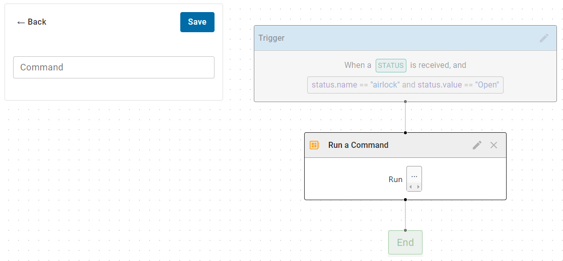
Step Builder
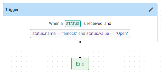
When you create a new workflow you are first presented with an empty Step Builder screen. It shows only the Trigger and End boxes in the workflow diagram, and the initial focus is on defining the Trigger.
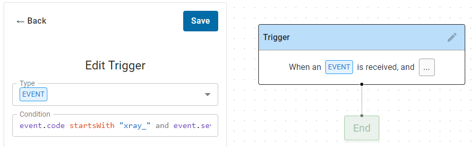
By default the trigger is set to an Event type, but you can select Manual (User_Dispatch), Metric or Status with the pull-down. For Event, Metric or Status type triggers, you then define the Condition. Default strings are inserted to give you some guidance and help you remember what to do.
- Type the condition
- As you type, syntactic suggestions are made.
- Select from the suggestions with the arrow keys.
- Add a suggestion to your condition with the tab key.
- Click Save to store your condition
- The Trigger box will be updated.
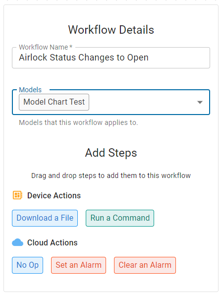
Then specify the workflow details at the left:
- Type in a name for the workflow.
- Select the Model that will use this workflow.
Note: Today you can select multiple models – this is a design issue that will be removed in a future release.
Note: Please select only a single model for each workflow. Why? Because there is only one copy of each workflow in the cloud. If you assign one workflow to multiple models, and in the future want to modify the workflow for just one of the models, you will have no way to easily do that.
Note: In a future version we will provide a way to create a copy of a workflow and reassign that copy to a different model. Then they can easily diverge.
Individual Steps
Within the workflow you can define the series of steps that will be executed to accomplish the goal. Order is important as the steps will be run in sequence, and no step will begin until the prior step and completed. Any step that fails will terminate the workflow.
| Step | Description | Parameters | Processing Location | Release |
|---|---|---|---|---|
| Run Command | Runs a single command line on the target device. | Command | Device | Mar 2023 |
| Set Device Tag | Sets the value of a Device Tag. | Device Tag Name | Cloud | ~Mar 2023 |
| Download File | Runs a single command line on the target device. | Command | Device | ~Apr 2023 |
| Set Alarm | Sets an alarm. | Alarm Name | Cloud | ~Apr 2023 |
| Clear Alarm | Clears an alarm. | Alarm Name | Cloud | ~Apr 2023 |
Defining the Workflow Steps.
To use the Step Builder:
- Drag (left mouse click and hold) a color step block from the Add Steps are at the left.
- As you drag one, you will see circled green plus signs appear indicating where you need to drag the block.
- Release the mouse click when the tip of the cursor is over the desired circle.
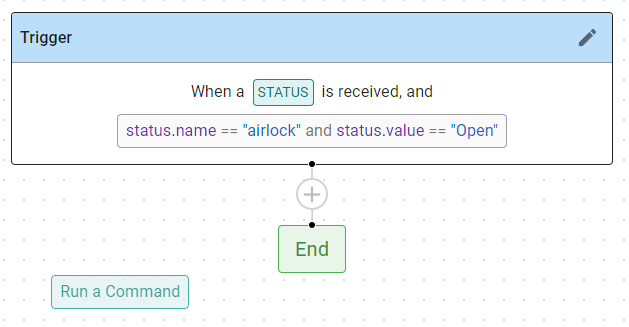
- If the step requires inputs, they will open by default at the left.
- Enter the required data for the step.
- Click Save to store the parameters for that step.
- Continue dragging and dropping step blocks onto the workflow diagram until all the steps are in place.
- When all the steps are in place, click Save (bottom left) to save the workflow.
4 - Device Health Indicators
Agent Status
The maiLink Agent will automatically send regular health updates to the cloud. These will be displayed in the maiLink UI as a circular icon. The icon meanings are described in the following table:
| Icon | Meaning |
|---|---|
| The Agent has sent a health update in the last 3 minutes | |
| The Agent has not sent a health update in the last 3 minutes | |
| The Agent has sent a health update in the last hour | |
| The Agent has never sent a health update |
App Status
Applications can provide heartbeat notifications via the Telemetry API. These will be displayed in the maiLink UI as a heart-shaped icon. The icon meanings are described in the following table:
| Icon | Meaning |
|---|---|
| Your application has reported a heartbeat in the last 3 minutes | |
| Your application has not reported a heartbeat in the last 3 minutes | |
| Your application has not reported a heartbeat in the last hour | |
| Your application has never reported a heartbeat telemetry event |
5 - maiLink Glossary
Basic Terms
These terms are best understood if read through in sequence.
| Term | Description |
|---|---|
| maiLink | The shorthand name for the maiLink SRM platform, the maiLink Apps that run on the maiLink SRM platform, and all of its features and capabilities. |
| Device | A manufactured product that is installed in the field. |
| Device Type | A class of manufactured products, such a those of the same make and model and, perhaps, with similar options. |
| Partner | A manufacturer or other business that is a direct user of maiLink SRM softare (E.g. they use it to track and monitor their products). |
| Customer | An entity that purchases and uses products manufactured by a maiLink Partner. |
maiLink Products
| Term | Description |
|---|---|
| maiLink SRM | The name of the maiData Service Relationship Management (SRM) software platform for tracking fleets of deployed devices and secure communications with those devices. |
| maiLink Apps | The collection of optional maiLink Apps are available on the maiLink SRM platform and can be enabled / disabled for each Device Type: |
maiLink Apps
| App | Description |
|---|---|
| Manage | This App allows Device Types to be created for each brand and model of product, and Devices to be created for each serial number. |
| Health | This App sends an “Agent Alive” health message from the Agent to the Cloud at a regular interval. |
| Access | This App provides secure remote access from an installed Client to deployed devices in the field. |
| Telemetry | This App sends asynchronous messages from the Agent to the Cloud. |
| Command | This App automates service tasks. Each Command is a script that combines individual file transfers to/from the device as well as remotely executed commands that are run on the device. Command allows scripts to be broadcast to one Device, a selected group of Deviecs (all of the same Device Type), or all the Devices of a Device Type. |
maiLink Telemetry Message Types
| Type | Description |
|---|---|
| Metrics | Numeric values that change over time. |
| Events | Momentary occurences on the Devices, such as “Door opened”, “System restarted”. Each Event has a Severity Level, a Code that identifies the type of Event, and a Descriptor that is human-readable. |
| Status | Describes the the current state of something in the Devices, such a “Door is Open” or “X-ray Tube is on”. Each Status has a Code that identifies the component being described, and a Descriptor that is human-readable. |
maiLink Software Components
| Type | Description |
|---|---|
| Agent | The maiLink software module built into products that can connect to the maiLink SRM software platform. |
| Client | The maiLink software module installed on Partner service technicians if/when they need to remotely access deployed Devices. |
| Cloud | The maiLink software cloud-based database, management, portal and secure communications software. |
| Router | A maiLink software accessory with built-in Agent that, when installed in a Customer facility and with the agreement of the Customer, allows the Partner to gain Access to non-maiLink compatible, network-connected systems. |
Types of Protected Information
These terms are usually used in the context of Information Security (SOC1, SOC2, SOC3, ISO-27001), Patient Privacy (HIPAA) and/or Data Protection (GDPR).
| Type | Description |
|---|---|
| PCI | Payment Card Information. |
| PHI | Payment Card Information. |
| PII | Payment Card Information. |
Other Terms
| Type | Description |
|---|---|
| PDLC | maiLink uses a Product Development Life Cycle process for developing maiLink products. |
| VA | In computing, a Virtual Appliance (VA) is considere a software equivalent of a hardware device, usually in the form of a preconfigured software solution. |
| VM | In computing, a Virtual Machine (VM) is the virtualization / emulation of a computer system. |